1. What Is Optimization?

Optimization is the process of finding the best solution among many possible alternatives while respecting a given set of conditions.

 

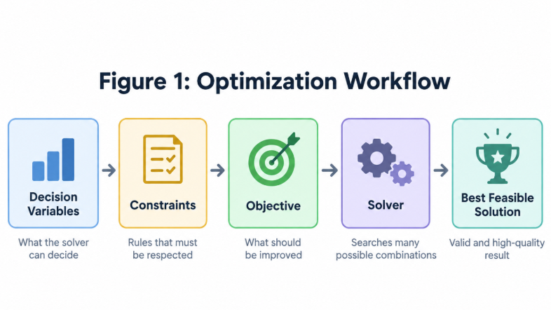
In software development, we often write rules that determine whether something is valid. Optimization goes one step further: instead of simply asking whether a solution is valid, we ask:

Among all valid solutions, which one is the best?

Consider a simple delivery example.

Suppose we have several delivery destinations and multiple vehicles. There may be many different ways to assign the deliveries to those vehicles.

For example, suppose there are 3 delivery plans like above:

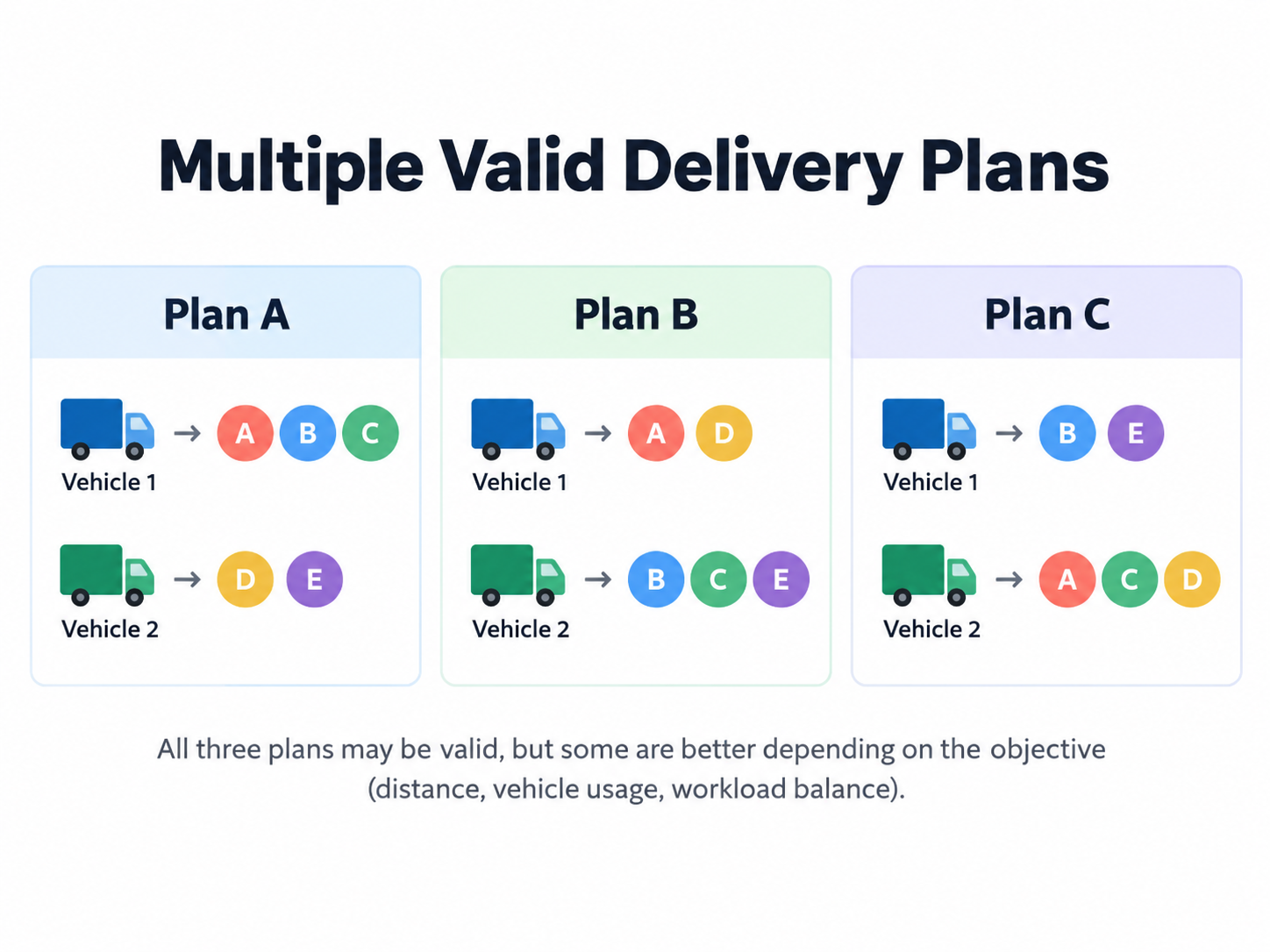
All three plans might be technically possible.

However, one plan may use fewer vehicles, another may result in a shorter total travel distance, and another may distribute the workload more evenly.

Optimization is about defining what a “good” solution means and then searching for a solution that performs well according to that definition.

In other words, an optimization problem usually has three important elements.

Those are: 1. Decision variables → 2. Constraints → Objective

For a delivery problem, a variable might represent:

Should destination A be assigned to Vehicle 1 or Vehicle 2?

The constraints define what is allowed.

For example:

A vehicle must not exceed its capacity.

The objective defines what we want to improve.

For example:

Minimize the total travel distance.

This is fundamentally different from simply writing a sequence of if statements.

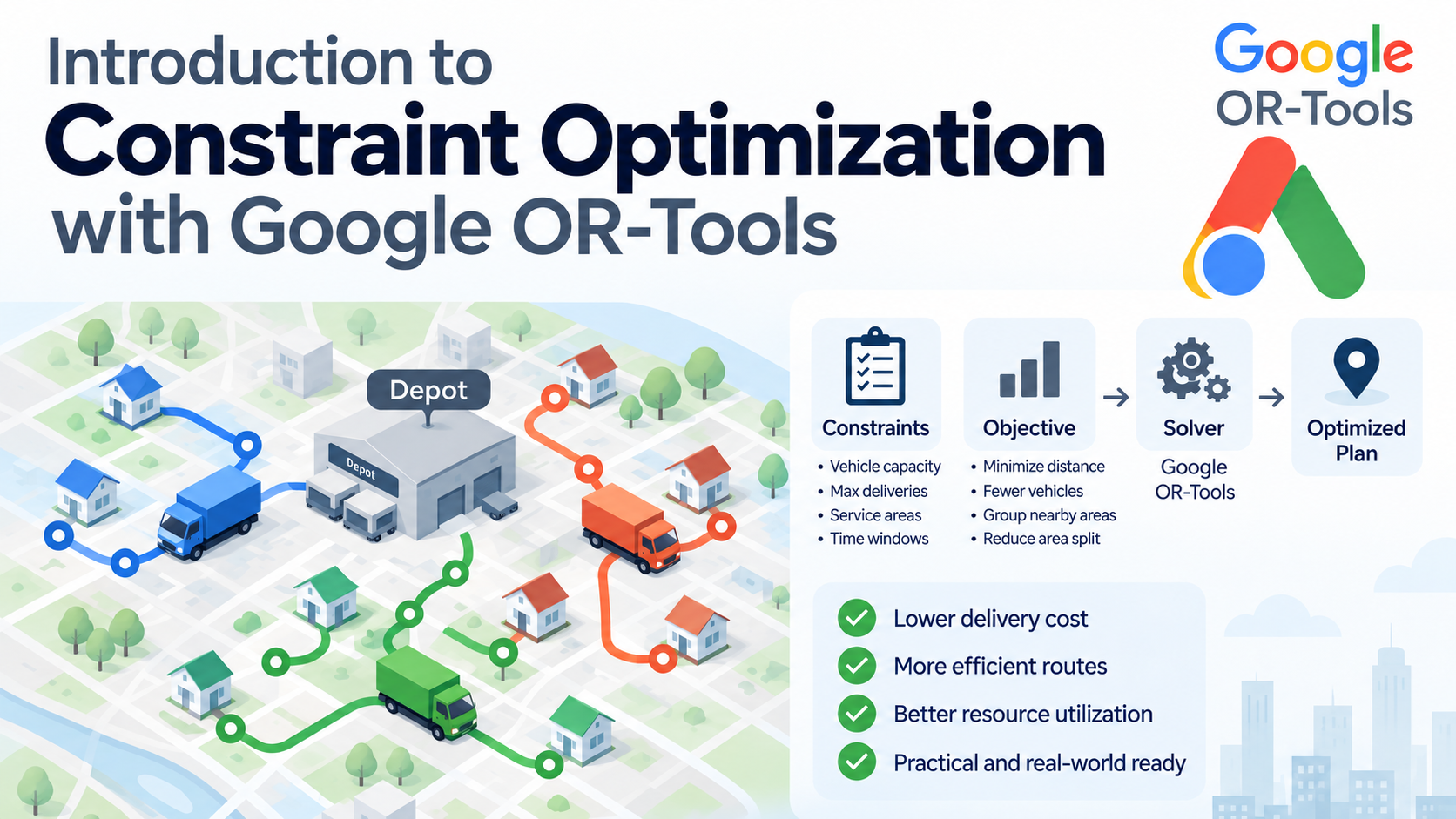
An optimization solver explores many possible combinations and searches for a solution that satisfies the constraints while improving the objective.

2. What Is a Constraint?

A constraint is a rule that defines which solutions are allowed.

Suppose a vehicle has a maximum capacity of 500 units.

If the total load assigned to that vehicle is 550 units, the assignment is not valid.

We can express the rule as:

Total assigned load ≤ 500

This is a constraint.

Optimization problems often contain many constraints at the same time.

For a delivery problem, they might include:

Vehicle capacity ≤ maximum capacity

Number of deliveries per vehicle ≤ daily limit

A delivery must be assigned to exactly one vehicle

A vehicle can only serve supported areas

The solver must find a solution that satisfies these rules.

There are two types of contraints: hard constraints and soft constraints. 

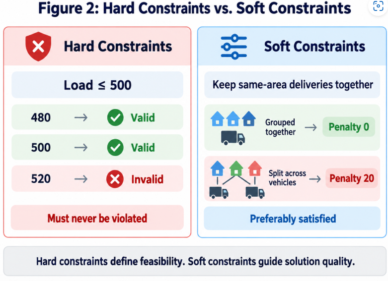
Hard Constraints

Some constraints must never be violated.

These are commonly called hard constraints.

For example:

Maximum vehicle capacity: 500

A solution with a load of 520 is simply invalid.

Load = 480 → Valid
Load = 500 → Valid
Load = 520 → Invalid

Hard constraints represent conditions that the system is not allowed to break.

Typical examples include:

• • maximum capacity

• • legal working-hour limits

• • vehicle compatibility

• • required delivery time windows

• • mandatory assignments

Soft Constraints

Other conditions may be desirable but not absolutely required.

These are often modeled as soft constraints.

For example:

Deliveries in the same geographical area should preferably be assigned to the same vehicle.

Breaking this preference may not make the plan impossible, but it may make the plan less desirable.

One way to model this is by assigning a penalty when the preference is violated.

For example:

Same-area deliveries grouped together
Penalty = 0

Same-area deliveries split across vehicles
Penalty = 20

The solver can then try to minimize the total penalty.

This distinction is important:

Hard Constraint
→ Must be satisfied

Soft Constraint
→ Preferably satisfied

The same business requirement can even be modeled differently depending on how strict it is.

For example:

“Vehicle utilization must never exceed 80%.”

could be modeled as a hard constraint.

But:

“We would prefer vehicle utilization to stay below 80%.”

could instead be modeled as a soft constraint with a penalty for exceeding the preferred level.

How a business rule is modeled therefore has a significant impact on the resulting solution.

3. What Is an Objective Function?

Constraints tell us which solutions are valid.

But they do not necessarily tell us which valid solution is the best.

Imagine that the solver finds three assignments, and all of them satisfy every constraint.

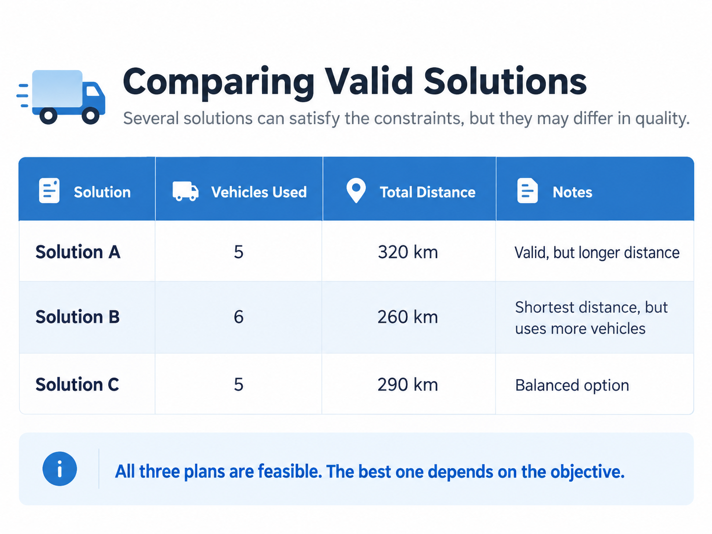
Which one should we choose?

The answer depends on what we are trying to optimize.

That is the role of the objective function.

An objective function assigns a value — often called a cost or score — to a solution.

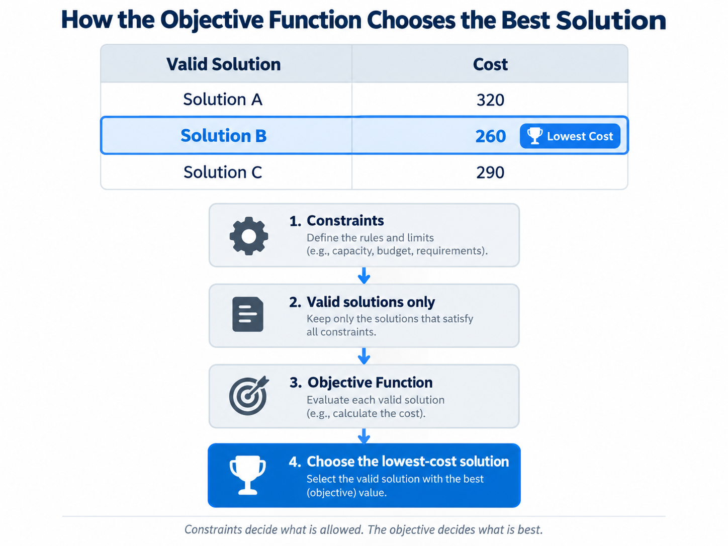
The solver then attempts to minimize or maximize that value.

For example:

Minimize total travel distance

could be expressed conceptually as:

Objective =
Distance traveled by Vehicle 1
+ Distance traveled by Vehicle 2
+ ...

The solver searches for a valid solution with the smallest objective value.

But distance is only one possible objective.

A logistics optimization problem might instead try to:

• • minimize the number of vehicles used

• • minimize total travel time

• • minimize transportation cost

• • balance workload between vehicles

• • reduce the number of split delivery areas

• • minimize penalties caused by undesirable assignments

Multiple factors can also be combined.

For example:

Objective =
    total_distance
  + vehicle_count × 1000
  + area_split_penalty × 100

The exact numbers here are only illustrative, but the idea is important.

By changing the weights, we change what the solver considers important.

For example, if using an additional vehicle is very expensive, we can give vehicle usage a high penalty.

If travel distance matters more, we can increase the weight of distance instead.

This is one of the most important concepts in optimization:

Constraints define what is possible.
The objective defines what is desirable.

A useful mental model is:

Constraints
"Can we do this?"

Objective
"How good is this solution?"

The optimization solver therefore performs two jobs at the same time:

1. Reject solutions that violate constraints.

2. Compare valid solutions using the objective function.

This combination of constraints + objective + search is the foundation of many optimization problems, including scheduling, resource allocation, manufacturing planning, workforce assignment, and vehicle routing.

The next step is to look at how Google OR-Tools provides the tools needed to model and solve these kinds of problems.

4. What Is Google OR-Tools?

Google OR-Tools is an open-source software suite developed by Google for solving optimization problems.

The name OR-Tools comes from Operations Research Tools.

Operations Research is a field focused on making better decisions when there are many possible choices, limited resources, and multiple constraints.

OR-Tools provides several different solvers and modeling tools for different types of optimization problems.

Typical use cases include:

• • vehicle routing

• • scheduling

• • workforce assignment

• • resource allocation

• • bin packing

• • production planning

• • network flow problems

OR-Tools is not a single optimization algorithm.

Instead, it is a collection of tools designed for different classes of problems.

Some of the major components include:

Routing Solver

The Routing Solver is designed for routing-related problems.

Typical examples include:

• • Traveling Salesman Problem (TSP)

• • Vehicle Routing Problem (VRP)

• • Capacitated Vehicle Routing Problem (CVRP)

• • Vehicle Routing Problem with Time Windows (VRPTW)

• • Pickup and Delivery problems

For example, if we have:

20 delivery locations
5 vehicles
vehicle capacity limits
delivery time windows

the Routing Solver can be used to search for an efficient assignment and route.

CP-SAT Solver

CP-SAT is a general-purpose constraint programming solver.

It is useful when a problem contains many discrete decisions and complex logical constraints.

For example:

Employee A cannot work on Monday.

Employee B must work either Tuesday or Wednesday.

At least two employees must be assigned to each shift.

These types of scheduling and assignment problems can often be modeled with CP-SAT.

Linear and Integer Optimization

OR-Tools also provides interfaces for linear programming and mixed-integer programming.

For example:

Maximize profit

subject to:

raw_material_usage ≤ available_material
labor_hours ≤ available_hours
production_quantity ≥ 0

These models are commonly used in production planning, resource allocation, and financial optimization.

The important point is that OR-Tools gives us a way to describe:

Variables
+
Constraints
+
Objective

and then lets the solver handle the difficult search process.

Instead of writing large amounts of custom logic such as:

if vehicle_1_has_capacity:
    assign_delivery()

elif vehicle_2_has_capacity:
    assign_delivery()

elif vehicle_3_has_capacity:
    ...

we describe the optimization problem itself.

The solver then searches through the possible combinations.

A simplified mental model is:

Problem definition
      ↓
Decision variables
      ↓
Constraints
      ↓
Objective
      ↓
Solver
      ↓
Solution

This separation is one of the major advantages of using an optimization framework.

As the number of business rules grows, the optimization model can often remain much easier to reason about than a large collection of procedural if / else rules.

5. What Is the Vehicle Routing Problem (VRP)?

The Vehicle Routing Problem, or VRP, is a classic optimization problem.

The basic question is:

How should multiple vehicles serve multiple locations efficiently?

Suppose we have one warehouse and several delivery locations.

                A
               /
Warehouse ---- B
   |          \
   |           C
   |
   +---------- D
               \
                E

We also have two vehicles.

The system needs to decide:

1. 1. which vehicle should visit each destination

1. 1. in what order each vehicle should visit its destinations

A possible solution might look like:

Vehicle 1
Warehouse → A → C → E → Warehouse

Vehicle 2
Warehouse → B → D → Warehouse

But many other combinations may also be possible.

The challenge is to find a good one.

VRP vs. TSP

A closely related problem is the Traveling Salesman Problem (TSP).

In a TSP, we usually have one traveler or one vehicle that must visit every location.

For example:

Warehouse
   ↓
A → C → D → B
   ↓
Warehouse

The goal might be to find the shortest possible route.

VRP extends this idea to multiple vehicles.

Instead of asking:

What is the best route for one vehicle?

we ask:

How should the destinations be divided among multiple vehicles, and what route should each vehicle take?

This makes the problem significantly more complex.

Real-World VRP Constraints

Real logistics problems usually contain additional constraints.

For example:

Vehicle Capacity

A vehicle cannot carry more than its maximum capacity.

Vehicle capacity = 500

Assigned load = 450 → Valid
Assigned load = 520 → Invalid

This variation is commonly called the Capacitated Vehicle Routing Problem (CVRP).

Time Windows

Some customers may only accept deliveries during specific periods.

Customer A
09:00 - 11:00

Customer B
13:00 - 15:00

The route must therefore satisfy both travel time and delivery time constraints.

This type of problem is commonly called VRP with Time Windows (VRPTW).

Different Vehicle Types

Vehicles may have different characteristics.

For example:

Vehicle 1
Capacity: 900
Area: Any

Vehicle 2
Capacity: 500
Area: East

Vehicle 3
Capacity: 300
Area: West

The solver must decide not only which route is efficient, but also whether each vehicle is eligible for the assigned destinations.

Maximum Number of Deliveries

A business may also impose operational limits such as:

Maximum 10 deliveries per vehicle per day

This constraint may not come directly from vehicle capacity.

It may instead reflect practical considerations such as:

• • unloading time

• • driver workload

• • customer waiting time

• • operational experience

The resulting optimization problem therefore becomes something like:

Assign every destination to a vehicle

while:

vehicle capacity is respected
delivery limits are respected
vehicle restrictions are respected

and:

total cost is minimized

This is exactly the kind of problem for which optimization libraries such as OR-Tools are useful.

A Simple VRP Model

Conceptually, a VRP can be thought of as three parts.

First, we have the inputs:

Vehicles
Destinations
Travel costs
Demand

Then we define the constraints:

Each destination must be served

Vehicle capacity must not be exceeded

Vehicle-specific restrictions must be respected

Finally, we define the objective:

Minimize total travel distance

or perhaps:

Minimize total operating cost

The solver then searches for a route assignment that satisfies the constraints while improving the objective.

As the number of destinations and constraints grows, the number of possible routes grows extremely quickly.

This is why solving a VRP is not simply a matter of checking every possible route one by one.

That leads naturally to the next topic: how optimization solvers search through an enormous number of possible solutions efficiently.

6. Conclusion

Constraint optimization provides a different way of thinking about software problems.

Instead of writing a fixed sequence of instructions that determines exactly what the program should do, we describe:

What can be decided?

What rules must be respected?

What makes one solution better than another?

These ideas correspond to the three core concepts introduced in this article:

Decision Variables
        ↓
Constraints
        ↓
Objective

The solver is then responsible for searching for a good solution.

Google OR-Tools provides a practical toolkit for building these kinds of optimization models.

It supports a wide range of problems, from scheduling and assignment to resource allocation and vehicle routing.

For routing problems in particular, the Vehicle Routing Problem provides a useful way to model real-world logistics requirements such as:

• • multiple vehicles

• • vehicle capacities

• • delivery restrictions

• • time windows

• • routing costs

The key idea is simple:

Constraints define what is allowed, while the objective defines what is preferred.

OR-Tools searches for solutions that satisfy the constraints while attempting to improve the objective.

However, one important question remains.

If a routing problem can contain millions — or even vastly more — possible combinations, how does OR-Tools actually search through them?

That is where concepts such as initial solutions, local search, neighborhood operators, and metaheuristics become important.

In the next article, we will look inside that search process and explore how OR-Tools moves from an initial feasible solution toward better ones.